3  Validación de constructos

Esta sección esta orientada a mostrar los análisis de consistencia interna entre los indicadores que conforman un constructo, para luego verificar la fiabilidad de su estructura teórica. Para ello, primero se calculará un análisis factorial exploratorio para cada subdimensión, tomando en cuenta todos los indicadores contabilizados en la propuesta anterior hecha con ELSOC (exceptuando el factor de seguridad, ya que este no tiene antecedentes en tal propuesta). A partir del número de factores encontrado en cada subdimensión, se estimarán análisis factoriales confirmatorios para corroborar si las construcciones propuestas funcionan correctamente.

4 Análisis factorial exploratorio

4.1 Factor seguridad

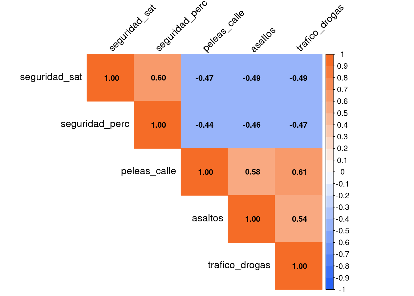
Se genera un subset de datos solamente con las variables que conforman el factor de seguridad para llevar a cabo el análisis.

elsoc_seg <- elsoc %>%
  select(seguridad_sat, seguridad_perc, peleas_calle, asaltos, trafico_drogas)

Las variables se convierten a numéricas.

elsoc_seg <- elsoc %>%
  select(seguridad_sat, seguridad_perc, peleas_calle, asaltos, trafico_drogas) %>%
  mutate(across(everything(), as.numeric))

Se calcula la matriz de correlaciones

corrplot(corrseg,
         method = "color",       # colorea los recuadros según valor
         col = colorRampPalette(c("#2761f5", "white", "#f56c27"))(20),  # blanco a rojo
         type = "upper",         # mostrar solo la mitad superior
         order = "original",     # mantener el orden de las variables
         addCoef.col = "black",  # añadir los valores numéricos
         tl.col = "black",       # color etiquetas
         tl.srt = 45, 
         bg = "white",# rotar etiquetas
         number.cex = 0.8
)

Figure 4.1: Correlaciones factor seguridad

KMO(corrseg) 

Kaiser-Meyer-Olkin factor adequacy
Call: KMO(r = corrseg)
Overall MSA =  0.83
MSA for each item = 
 seguridad_sat seguridad_perc   peleas_calle        asaltos trafico_drogas 
          0.82           0.82           0.82           0.86           0.84 

cortest.bartlett(corrseg, n = 2730)

$chisq
[1] 5182.035

$p.value
[1] 0

$df
[1] 10

Ya con la matriz de correlaciones lista, pasamos a realizar el EFA

Parallel analysis suggests that the number of factors =  2  and the number of components =  NA 

Factor Analysis

	Factor 1	Factor 2	Communality
seguridad_sat	-0.35	0.72	0.63
seguridad_perc	-0.32	0.69	0.57
peleas_calle	0.78	-0.27	0.69
asaltos	0.60	-0.39	0.51
trafico_drogas	0.65	-0.38	0.56
Total Communalities			2.97
Cronbach's α	0.80	0.75

Table 4.1: Análisis factorial exploratorio del factor seguridad

En Table 1 se puede apreciar que el factorial exploratorio reconoce la existencia de dos factores latentes. Uno de ellos puede comprenderse como seguridad subjetiva, el cual integra los indicadores de satisfacción de seguridad y percepción de seguridad. Ambos indicadores poseen cargas factoriales altas, así como un alfa de Cronbach aceptable, por lo que es un factor consistente. El segundo factor contiene los indicadores de frecuencia de conflictos en el barrio, por lo que pueden agruparse bajo el factor de seguridad objetiva. El factor explica en buena medida as cargas factoriales de los tres indicadores en tanto rondan entre .6 y .8. Su alfa de Cronbach refleja una buena consistencia entre los indicadores de seguridad objetiva.

4.2 Factor de calidad de vida en el vecindario

Subset con los indicadores necesarios

elsoc_barrio <- elsoc %>%
  select(confianza_vecinos, barrio_ideal, barrio_integracion, barrio_identidad,
         barrio_pertenencia, barrio_amigos, barrio_sociable, barrio_cordial,
         barrio_colaborador, conectividad, areas_verdes, barrio_limpio,
         cercania_actividad, cercania_escuelas, cercania_comercio,
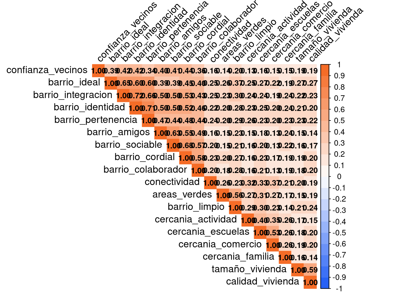
         cercania_familia, tamaño_vivienda, calidad_vivienda)

Las variables se convierten a numéricas

elsoc_barrio <- elsoc %>%
  select(confianza_vecinos, barrio_ideal, barrio_integracion, barrio_identidad,
         barrio_pertenencia, barrio_amigos, barrio_sociable, barrio_cordial,
         barrio_colaborador, conectividad, areas_verdes, barrio_limpio,
         cercania_actividad, cercania_escuelas, cercania_comercio,
         cercania_familia, tamaño_vivienda, calidad_vivienda) %>%
  mutate(across(everything(), as.numeric))

Se calcula la matriz de correlaciones

corrplot(corrbarrio,
         method = "color",       # colorea los recuadros según valor
         col = colorRampPalette(c("#2761f5", "white", "#f56c27"))(20),  # blanco a rojo
         type = "upper",         # mostrar solo la mitad superior
         order = "original",     # mantener el orden de las variables
         addCoef.col = "black",  # añadir los valores numéricos
         tl.col = "black",       # color etiquetas
         tl.srt = 45, 
         bg = "white",# rotar etiquetas
         number.cex = 0.8
)

Figure 4.2: Correlaciones factor calidad de vida en el barrio

KMO(corrbarrio) 

Kaiser-Meyer-Olkin factor adequacy
Call: KMO(r = corrbarrio)
Overall MSA =  0.9
MSA for each item = 
 confianza_vecinos       barrio_ideal barrio_integracion   barrio_identidad 
              0.96               0.94               0.92               0.92 
barrio_pertenencia      barrio_amigos    barrio_sociable     barrio_cordial 
              0.92               0.93               0.89               0.92 
barrio_colaborador       conectividad       areas_verdes      barrio_limpio 
              0.95               0.93               0.81               0.84 
cercania_actividad  cercania_escuelas  cercania_comercio   cercania_familia 
              0.91               0.86               0.84               0.94 
   tamaño_vivienda   calidad_vivienda 
              0.76               0.76 

cortest.bartlett(corrbarrio, n = 2730)

$chisq
[1] 19599.6

$p.value
[1] 0

$df
[1] 153

Parallel analysis suggests that the number of factors =  5  and the number of components =  NA 

Factor Analysis

	Factor 1	Factor 2	Factor 3	Factor 4	Factor 5	Communality
confianza_vecinos	0.43	0.29	0.11	0.13	0.07	0.30
barrio_ideal	0.29	0.61	0.20	0.17	0.21	0.57
barrio_integracion	0.40	0.70	0.18	0.10	0.11	0.70
barrio_identidad	0.40	0.73	0.18	0.07	0.06	0.73
barrio_pertenencia	0.34	0.70	0.18	0.10	0.09	0.65
barrio_amigos	0.66	0.29	0.11	0.04	0.07	0.53
barrio_sociable	0.82	0.19	0.12	0.05	0.03	0.73
barrio_cordial	0.73	0.26	0.15	0.09	0.11	0.64
barrio_colaborador	0.62	0.23	0.12	0.09	0.14	0.48
conectividad	0.13	0.12	0.46	0.12	0.12	0.27
areas_verdes	0.09	0.09	0.30	0.07	0.57	0.44
barrio_limpio	0.15	0.16	0.20	0.12	0.81	0.76
cercania_actividad	0.06	0.15	0.50	0.06	0.18	0.31
cercania_escuelas	0.11	0.08	0.68	0.07	0.16	0.51
cercania_comercio	0.03	0.06	0.71	0.10	0.08	0.53
cercania_familia	0.18	0.13	0.35	0.08	0.02	0.18
tamaño_vivienda	0.09	0.12	0.16	0.74	0.06	0.60
calidad_vivienda	0.10	0.10	0.16	0.72	0.11	0.58
Total Communalities						9.53
Cronbach's α	0.83	0.88	0.71	0.74	0.72

Table 4.2: Análisis factorial exploratorio del vinculación territorial

4.3 Factor redes sociales (ola 5)

Seleccionamos las variables a utilizar

elsoc_redes <- elsoc_redes %>%
select(confianza_gen, altruismo_gen, visitar_vecino,
       reunion_pub, visita_amigos, voluntariado, donar_dinero, prestar_dinero, 
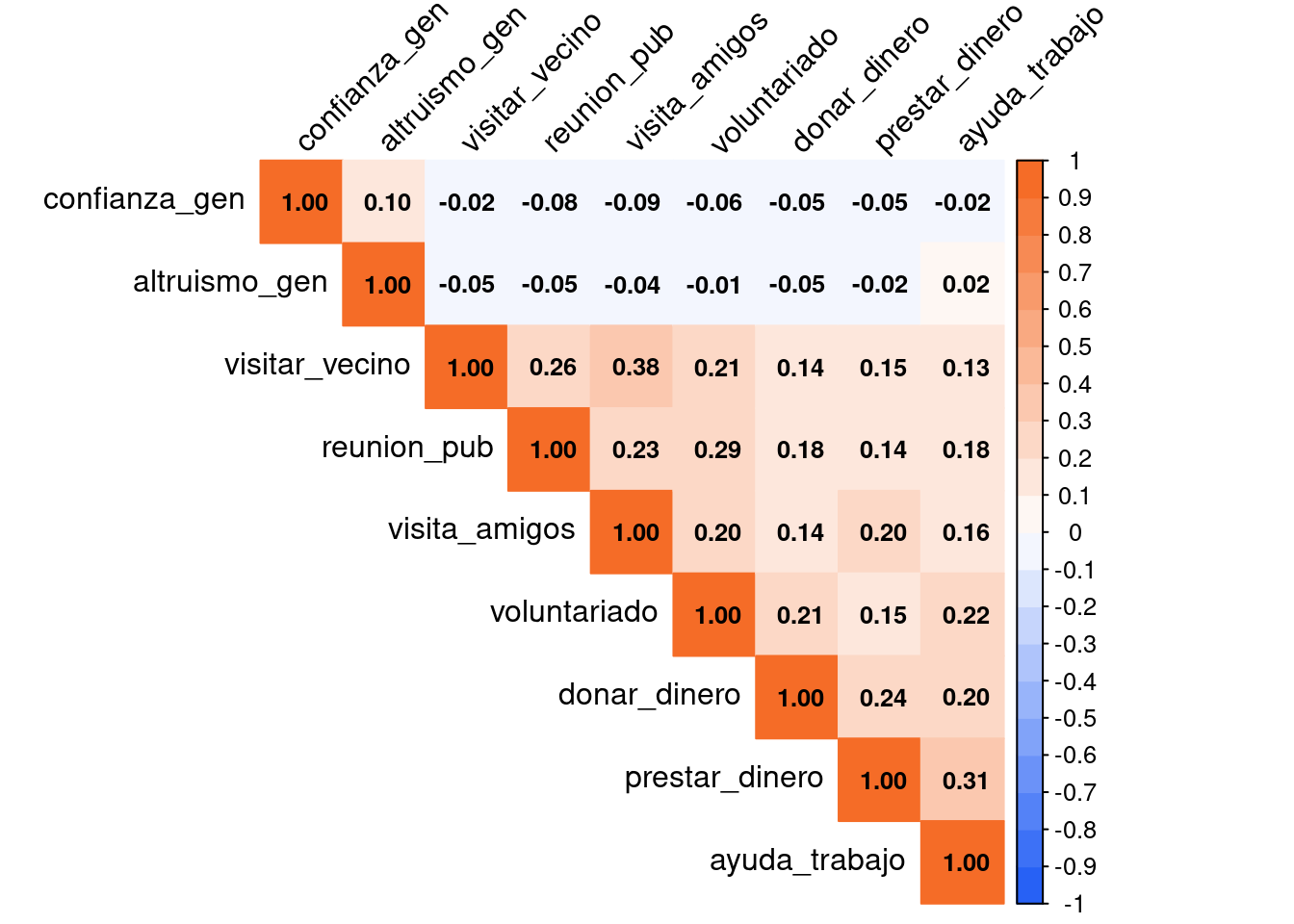
       ayuda_trabajo)

Pasamos las variables a numéricas

elsoc_redes <- elsoc_redes %>%
  select(confianza_gen, altruismo_gen, visitar_vecino,
       reunion_pub, visita_amigos, voluntariado, donar_dinero, prestar_dinero, 
       ayuda_trabajo) %>%
  mutate(across(everything(), as.numeric))

hist(elsoc_redes$confianza_gen,main="Histograma del Vector",xlab="Valor",ylab="Frecuencia",col="cyan4",border="black")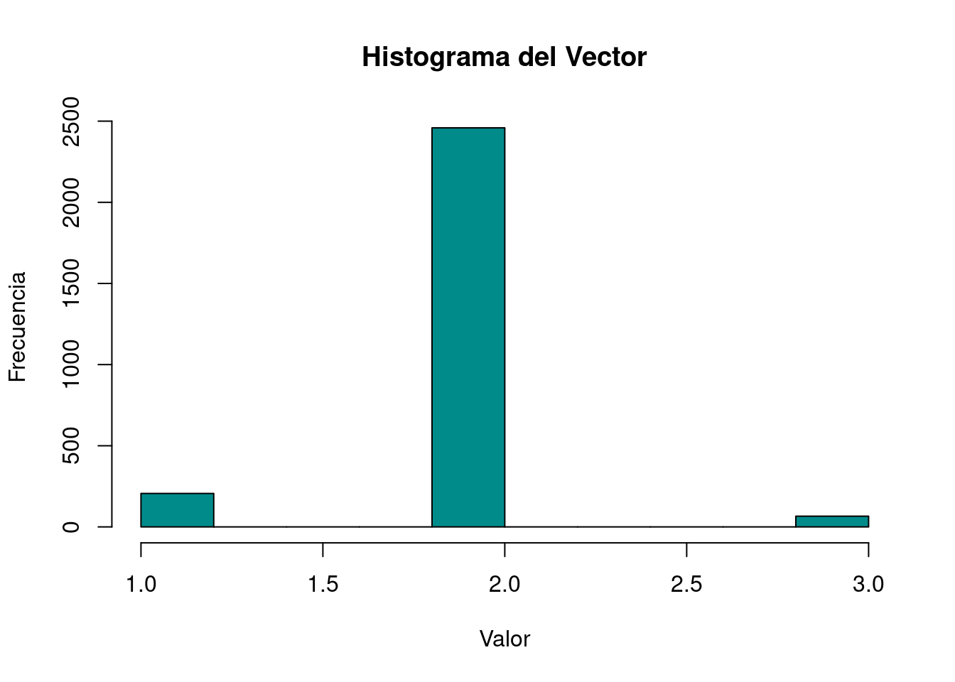

elsoc_redes$confianza_gen <- car::recode(elsoc_redes$confianza_gen, "c(1, 3)= 0; (2)=1")

Estimamos la matriz de correlaciones

corrplot(corredes,
         method = "color",       # colorea los recuadros según valor
         col = colorRampPalette(c("#2761f5", "white", "#f56c27"))(20),  
         type = "upper",         # mostrar solo la mitad superior
         order = "original",     # mantener el orden de las variables
         addCoef.col = "black",  # añadir los valores numéricos
         tl.col = "black",       # color etiquetas
         tl.srt = 45, 
         bg = "white",# rotar etiquetas
         number.cex = 0.8
)

Figure 4.3: Correlaciones factor redes sociales

KMO(corredes) 

Kaiser-Meyer-Olkin factor adequacy
Call: KMO(r = corredes)
Overall MSA =  0.73
MSA for each item = 
 confianza_gen  altruismo_gen visitar_vecino    reunion_pub  visita_amigos 
          0.63           0.58           0.70           0.77           0.71 
  voluntariado   donar_dinero prestar_dinero  ayuda_trabajo 
          0.77           0.78           0.72           0.73 

cortest.bartlett(corredes, n = 2740)

$chisq
[1] 1991.963

$p.value
[1] 0

$df
[1] 36

Parallel analysis suggests that the number of factors =  4  and the number of components =  NA 

Factor Analysis

	Factor 1	Factor 2	Factor 3	Factor 4	Communality
confianza_gen	0.00	-0.04	-0.06	0.39	0.16
altruismo_gen	-0.05	0.00	-0.01	0.25	0.06
visitar_vecino	0.77	0.07	0.18	-0.02	0.63
reunion_pub	0.22	0.11	0.44	-0.13	0.27
visita_amigos	0.42	0.18	0.21	-0.15	0.28
voluntariado	0.13	0.13	0.56	-0.03	0.34
donar_dinero	0.09	0.29	0.28	-0.06	0.17
prestar_dinero	0.11	0.71	0.07	-0.06	0.52
ayuda_trabajo	0.07	0.40	0.29	0.05	0.26
Total Communalities					2.70
Cronbach's α	0.55	0.50	0.45	0.16

Table 4.3: Análisis factorial exploratorio del factor redes sociales

5 Análisis factorial confirmatorio

5.1 Factor seguridad

Especificamos el modelo tomando en cuenta la propuesta teórica del documento.

seguridad_model <- '
subjetiva =~ seguridad_perc + seguridad_sat
objetiva =~ peleas_calle + asaltos + trafico_drogas
'

Se estima el modelo

seguridad_cfa <- cfa(model = seguridad_model,
                     data = elsoc_seg,
                     estimator = "WLSMV",
                     ordered = TRUE,
                     std.lv = FALSE)

Visualizamos los resultados

summary(seguridad_cfa, standardized = TRUE, fit.measures = TRUE)

lavaan 0.6-19 ended normally after 18 iterations

  Estimator                                       DWLS
  Optimization method                           NLMINB
  Number of model parameters                        26

                                                  Used       Total
  Number of observations                          2403        2730

Model Test User Model:
                                              Standard      Scaled
  Test Statistic                                10.109      27.370
  Degrees of freedom                                 4           4
  P-value (Chi-square)                           0.039       0.000
  Scaling correction factor                                  0.372
  Shift parameter                                            0.220
    simple second-order correction                                

Model Test Baseline Model:

  Test statistic                             18024.644   11961.968
  Degrees of freedom                                10          10
  P-value                                        0.000       0.000
  Scaling correction factor                                  1.507

User Model versus Baseline Model:

  Comparative Fit Index (CFI)                    1.000       0.998
  Tucker-Lewis Index (TLI)                       0.999       0.995
                                                                  
  Robust Comparative Fit Index (CFI)                         0.996
  Robust Tucker-Lewis Index (TLI)                            0.989

Root Mean Square Error of Approximation:

  RMSEA                                          0.025       0.049
  90 Percent confidence interval - lower         0.005       0.033
  90 Percent confidence interval - upper         0.045       0.068
  P-value H_0: RMSEA <= 0.050                    0.982       0.487
  P-value H_0: RMSEA >= 0.080                    0.000       0.002
                                                                  
  Robust RMSEA                                               0.052
  90 Percent confidence interval - lower                     0.033
  90 Percent confidence interval - upper                     0.072
  P-value H_0: Robust RMSEA <= 0.050                         0.402
  P-value H_0: Robust RMSEA >= 0.080                         0.011

Standardized Root Mean Square Residual:

  SRMR                                           0.012       0.012

Parameter Estimates:

  Parameterization                               Delta
  Standard errors                           Robust.sem
  Information                                 Expected
  Information saturated (h1) model        Unstructured

Latent Variables:
                   Estimate  Std.Err  z-value  P(>|z|)   Std.lv  Std.all
  subjetiva =~                                                          
    seguridad_perc    1.000                               0.786    0.786
    seguridad_sat     1.051    0.026   40.455    0.000    0.826    0.826
  objetiva =~                                                           
    peleas_calle      1.000                               0.842    0.842
    asaltos           0.933    0.016   56.583    0.000    0.785    0.785
    trafico_drogas    0.967    0.017   58.072    0.000    0.814    0.814

Covariances:
                   Estimate  Std.Err  z-value  P(>|z|)   Std.lv  Std.all
  subjetiva ~~                                                          
    objetiva         -0.533    0.015  -36.666    0.000   -0.806   -0.806

Thresholds:
                   Estimate  Std.Err  z-value  P(>|z|)   Std.lv  Std.all
    segurdd_prc|t1   -1.679    0.044  -38.053    0.000   -1.679   -1.679
    segurdd_prc|t2   -0.766    0.028  -26.885    0.000   -0.766   -0.766
    segurdd_prc|t3   -0.190    0.026   -7.399    0.000   -0.190   -0.190
    segurdd_prc|t4    1.257    0.034   36.476    0.000    1.257    1.257
    seguridd_st|t1   -1.603    0.042  -38.216    0.000   -1.603   -1.603
    seguridd_st|t2   -0.569    0.027  -20.972    0.000   -0.569   -0.569
    seguridd_st|t3   -0.099    0.026   -3.854    0.000   -0.099   -0.099
    seguridd_st|t4    1.400    0.037   37.707    0.000    1.400    1.400
    peleas_call|t1   -0.059    0.026   -2.305    0.021   -0.059   -0.059
    peleas_call|t2    0.632    0.028   22.953    0.000    0.632    0.632
    peleas_call|t3    1.176    0.033   35.460    0.000    1.176    1.176
    peleas_call|t4    1.846    0.050   37.072    0.000    1.846    1.846
    asaltos|t1       -0.453    0.027  -17.048    0.000   -0.453   -0.453
    asaltos|t2        0.299    0.026   11.506    0.000    0.299    0.299
    asaltos|t3        0.973    0.031   31.910    0.000    0.973    0.973
    asaltos|t4        1.791    0.048   37.482    0.000    1.791    1.791
    trafic_drgs|t1   -0.264    0.026  -10.207    0.000   -0.264   -0.264
    trafic_drgs|t2    0.163    0.026    6.340    0.000    0.163    0.163
    trafic_drgs|t3    0.564    0.027   20.813    0.000    0.564    0.564
    trafic_drgs|t4    1.176    0.033   35.460    0.000    1.176    1.176

Variances:
                   Estimate  Std.Err  z-value  P(>|z|)   Std.lv  Std.all
   .seguridad_perc    0.382                               0.382    0.382
   .seguridad_sat     0.317                               0.317    0.317
   .peleas_calle      0.292                               0.292    0.292
   .asaltos           0.384                               0.384    0.384
   .trafico_drogas    0.338                               0.338    0.338
    subjetiva         0.618    0.020   31.175    0.000    1.000    1.000
    objetiva          0.708    0.017   41.904    0.000    1.000    1.000

Cargas factoriales estandarizadas

standardizedSolution(seguridad_cfa) %>% 
  dplyr::filter(op == "=~") %>% 
  dplyr::select(lhs, rhs, est.std)

        lhs            rhs est.std
1 subjetiva seguridad_perc   0.786
2 subjetiva  seguridad_sat   0.826
3  objetiva   peleas_calle   0.842
4  objetiva        asaltos   0.785
5  objetiva trafico_drogas   0.814

En este modelo todas las cargas factoriales estandarizadas son altas, donde los cinco indicadores oscilan entre el 0.7 y 0.8. Todos los indicadores son explicados en buena medida por su factor latente respectivo.

5.2 Factor vinculación territorial

Después de haber visto los EFA, sumado a la idea de realizar una propuesta minimalista de cohesión social, es que se propone modificar la subdimensión de “calidad de vida en el vecindario” y llamarla “vinculación territorial”, la cual estaría compuesta por un factor de sentido de pertenencia territorial y otro de satisfacción con el barrio.

barrio_model <- '
pertenencia =~ barrio_ideal + barrio_integracion + barrio_identidad + barrio_pertenencia
satisfaccion =~ barrio_amigos + barrio_sociable + barrio_cordial + barrio_colaborador
'

Estimación del modelo

barrio_cfa <- cfa(model = barrio_model,
                     data = elsoc_barrio,
                     estimator = "WLSMV",
                     ordered = TRUE,
                     std.lv = FALSE)

summary(barrio_cfa, standardized = TRUE, fit.measures = TRUE)

lavaan 0.6-19 ended normally after 23 iterations

  Estimator                                       DWLS
  Optimization method                           NLMINB
  Number of model parameters                        41

                                                  Used       Total
  Number of observations                          2525        2730

Model Test User Model:
                                              Standard      Scaled
  Test Statistic                               109.585     259.088
  Degrees of freedom                                19          19
  P-value (Chi-square)                           0.000       0.000
  Scaling correction factor                                  0.428
  Shift parameter                                            3.101
    simple second-order correction                                

Model Test Baseline Model:

  Test statistic                             96965.694   40795.676
  Degrees of freedom                                28          28
  P-value                                        0.000       0.000
  Scaling correction factor                                  2.378

User Model versus Baseline Model:

  Comparative Fit Index (CFI)                    0.999       0.994
  Tucker-Lewis Index (TLI)                       0.999       0.991
                                                                  
  Robust Comparative Fit Index (CFI)                         0.980
  Robust Tucker-Lewis Index (TLI)                            0.971

Root Mean Square Error of Approximation:

  RMSEA                                          0.043       0.071
  90 Percent confidence interval - lower         0.036       0.063
  90 Percent confidence interval - upper         0.052       0.079
  P-value H_0: RMSEA <= 0.050                    0.907       0.000
  P-value H_0: RMSEA >= 0.080                    0.000       0.025
                                                                  
  Robust RMSEA                                               0.079
  90 Percent confidence interval - lower                     0.072
  90 Percent confidence interval - upper                     0.088
  P-value H_0: Robust RMSEA <= 0.050                         0.000
  P-value H_0: Robust RMSEA >= 0.080                         0.463

Standardized Root Mean Square Residual:

  SRMR                                           0.021       0.021

Parameter Estimates:

  Parameterization                               Delta
  Standard errors                           Robust.sem
  Information                                 Expected
  Information saturated (h1) model        Unstructured

Latent Variables:
                   Estimate  Std.Err  z-value  P(>|z|)   Std.lv  Std.all
  pertenencia =~                                                        
    barrio_ideal      1.000                               0.780    0.780
    barrio_intgrcn    1.138    0.013   86.330    0.000    0.887    0.887
    barrio_identdd    1.149    0.013   88.538    0.000    0.896    0.896
    barrio_pertnnc    1.105    0.013   85.890    0.000    0.861    0.861
  satisfaccion =~                                                       
    barrio_amigos     1.000                               0.791    0.791
    barrio_sociabl    1.102    0.014   80.348    0.000    0.872    0.872
    barrio_cordial    1.118    0.013   82.957    0.000    0.885    0.885
    barrio_colbrdr    0.962    0.014   67.989    0.000    0.761    0.761

Covariances:
                   Estimate  Std.Err  z-value  P(>|z|)   Std.lv  Std.all
  pertenencia ~~                                                        
    satisfaccion      0.472    0.011   42.483    0.000    0.765    0.765

Thresholds:
                   Estimate  Std.Err  z-value  P(>|z|)   Std.lv  Std.all
    barrio_idel|t1   -1.982    0.054  -36.608    0.000   -1.982   -1.982
    barrio_idel|t2   -0.999    0.030  -33.260    0.000   -0.999   -0.999
    barrio_idel|t3   -0.572    0.026  -21.604    0.000   -0.572   -0.572
    barrio_idel|t4    1.023    0.030   33.728    0.000    1.023    1.023
    barr_ntgrcn|t1   -2.042    0.057  -35.847    0.000   -2.042   -2.042
    barr_ntgrcn|t2   -1.138    0.032  -35.784    0.000   -1.138   -1.138
    barr_ntgrcn|t3   -0.642    0.027  -23.844    0.000   -0.642   -0.642
    barr_ntgrcn|t4    1.048    0.031   34.221    0.000    1.048    1.048
    barri_dntdd|t1   -2.050    0.057  -35.739    0.000   -2.050   -2.050
    barri_dntdd|t2   -1.001    0.030  -33.293    0.000   -1.001   -1.001
    barri_dntdd|t3   -0.479    0.026  -18.405    0.000   -0.479   -0.479
    barri_dntdd|t4    1.079    0.031   34.799    0.000    1.079    1.079
    barr_prtnnc|t1   -2.110    0.060  -34.885    0.000   -2.110   -2.110
    barr_prtnnc|t2   -1.090    0.031  -34.988    0.000   -1.090   -1.090
    barr_prtnnc|t3   -0.609    0.027  -22.804    0.000   -0.609   -0.609
    barr_prtnnc|t4    1.003    0.030   33.327    0.000    1.003    1.003
    barrio_amgs|t1   -1.868    0.049  -37.809    0.000   -1.868   -1.868
    barrio_amgs|t2   -0.790    0.028  -28.232    0.000   -0.790   -0.790
    barrio_amgs|t3   -0.121    0.025   -4.834    0.000   -0.121   -0.121
    barrio_amgs|t4    1.397    0.036   38.634    0.000    1.397    1.397
    barrio_scbl|t1   -2.119    0.061  -34.747    0.000   -2.119   -2.119
    barrio_scbl|t2   -1.058    0.031  -34.415    0.000   -1.058   -1.058
    barrio_scbl|t3   -0.412    0.026  -16.009    0.000   -0.412   -0.412
    barrio_scbl|t4    1.310    0.035   37.951    0.000    1.310    1.310
    barrio_crdl|t1   -2.148    0.063  -34.307    0.000   -2.148   -2.148
    barrio_crdl|t2   -1.205    0.033  -36.757    0.000   -1.205   -1.205
    barrio_crdl|t3   -0.578    0.027  -21.798    0.000   -0.578   -0.578
    barrio_crdl|t4    1.254    0.034   37.360    0.000    1.254    1.254
    barr_clbrdr|t1   -1.989    0.054  -36.522    0.000   -1.989   -1.989
    barr_clbrdr|t2   -1.058    0.031  -34.415    0.000   -1.058   -1.058
    barr_clbrdr|t3   -0.388    0.026  -15.141    0.000   -0.388   -0.388
    barr_clbrdr|t4    1.203    0.033   36.729    0.000    1.203    1.203

Variances:
                   Estimate  Std.Err  z-value  P(>|z|)   Std.lv  Std.all
   .barrio_ideal      0.392                               0.392    0.392
   .barrio_intgrcn    0.213                               0.213    0.213
   .barrio_identdd    0.197                               0.197    0.197
   .barrio_pertnnc    0.258                               0.258    0.258
   .barrio_amigos     0.374                               0.374    0.374
   .barrio_sociabl    0.240                               0.240    0.240
   .barrio_cordial    0.217                               0.217    0.217
   .barrio_colbrdr    0.421                               0.421    0.421
    pertenencia       0.608    0.013   45.550    0.000    1.000    1.000
    satisfaccion      0.626    0.014   45.405    0.000    1.000    1.000

Cargas factoriales estandarizadas

standardizedSolution(barrio_cfa) %>% 
  dplyr::filter(op == "=~") %>% 
  dplyr::select(lhs, rhs, est.std)

           lhs                rhs est.std
1  pertenencia       barrio_ideal   0.780
2  pertenencia barrio_integracion   0.887
3  pertenencia   barrio_identidad   0.896
4  pertenencia barrio_pertenencia   0.861
5 satisfaccion      barrio_amigos   0.791
6 satisfaccion    barrio_sociable   0.872
7 satisfaccion     barrio_cordial   0.885
8 satisfaccion barrio_colaborador   0.761

Todas las cargas factoriales son altas, rondando entre en 0.7 y 0.8, por lo que ambos factores estarían explicando consistentemente sus indicadores correspondientes.

5.3 Factor redes sociales

A partir del EFA y la idea de minimalizar la propuesta, se decide plantear un modelo con tres factores: confianza interpersonal, comportamiento prosocial y apoyo económico. Se reduce la cantidad de indicadores de 10 a 6, dos pertenecientes a cada factor.

redes_model_conf <- '
confianza_inter =~ confianza_gen + altruismo_gen
prosocial =~ reunion_pub + voluntariado
economica =~ prestar_dinero + ayuda_trabajo
'

redes_conf_cfa <- cfa(model = redes_model_conf,
                     data = elsoc_redes,
                     estimator = "WLSMV",
                     ordered = TRUE,
                     std.lv = FALSE)

summary(redes_conf_cfa, standardized = TRUE, fit.measures = TRUE)

lavaan 0.6-19 ended normally after 37 iterations

  Estimator                                       DWLS
  Optimization method                           NLMINB
  Number of model parameters                        20

                                                  Used       Total
  Number of observations                          2723        2740

Model Test User Model:
                                              Standard      Scaled
  Test Statistic                                10.369      14.541
  Degrees of freedom                                 6           6
  P-value (Chi-square)                           0.110       0.024
  Scaling correction factor                                  0.720
  Shift parameter                                            0.139
    simple second-order correction                                

Model Test Baseline Model:

  Test statistic                              1111.820    1015.178
  Degrees of freedom                                15          15
  P-value                                        0.000       0.000
  Scaling correction factor                                  1.097

User Model versus Baseline Model:

  Comparative Fit Index (CFI)                    0.996       0.991
  Tucker-Lewis Index (TLI)                       0.990       0.979
                                                                  
  Robust Comparative Fit Index (CFI)                         0.985
  Robust Tucker-Lewis Index (TLI)                            0.963

Root Mean Square Error of Approximation:

  RMSEA                                          0.016       0.023
  90 Percent confidence interval - lower         0.000       0.008
  90 Percent confidence interval - upper         0.033       0.038
  P-value H_0: RMSEA <= 0.050                    1.000       0.999
  P-value H_0: RMSEA >= 0.080                    0.000       0.000
                                                                  
  Robust RMSEA                                               0.040
  90 Percent confidence interval - lower                     0.005
  90 Percent confidence interval - upper                     0.070
  P-value H_0: Robust RMSEA <= 0.050                         0.674
  P-value H_0: Robust RMSEA >= 0.080                         0.012

Standardized Root Mean Square Residual:

  SRMR                                           0.023       0.023

Parameter Estimates:

  Parameterization                               Delta
  Standard errors                           Robust.sem
  Information                                 Expected
  Information saturated (h1) model        Unstructured

Latent Variables:
                     Estimate  Std.Err  z-value  P(>|z|)   Std.lv  Std.all
  confianza_inter =~                                                      
    confianza_gen       1.000                               0.749    0.749
    altruismo_gen       0.270    0.167    1.614    0.107    0.202    0.202
  prosocial =~                                                            
    reunion_pub         1.000                               0.614    0.614
    voluntariado        1.191    0.115   10.384    0.000    0.731    0.731
  economica =~                                                            
    prestar_dinero      1.000                               0.564    0.564
    ayuda_trabajo       1.300    0.132    9.867    0.000    0.733    0.733

Covariances:
                     Estimate  Std.Err  z-value  P(>|z|)   Std.lv  Std.all
  confianza_inter ~~                                                      
    prosocial          -0.136    0.033   -4.179    0.000   -0.297   -0.297
    economica          -0.053    0.027   -1.964    0.050   -0.125   -0.125
  prosocial ~~                                                            
    economica           0.216    0.024    8.876    0.000    0.623    0.623

Thresholds:
                   Estimate  Std.Err  z-value  P(>|z|)   Std.lv  Std.all
    confianz_gn|t1   -1.286    0.033  -39.166    0.000   -1.286   -1.286
    altruism_gn|t1   -0.902    0.028  -32.281    0.000   -0.902   -0.902
    altruism_gn|t2    1.497    0.037   40.586    0.000    1.497    1.497
    reunion_pub|t1    0.662    0.026   25.411    0.000    0.662    0.662
    reunion_pub|t2    1.233    0.032   38.546    0.000    1.233    1.233
    voluntariad|t1    0.745    0.027   28.005    0.000    0.745    0.745
    voluntariad|t2    1.082    0.030   36.192    0.000    1.082    1.082
    prestar_dnr|t1   -0.556    0.025  -21.880    0.000   -0.556   -0.556
    prestar_dnr|t2    0.015    0.024    0.632    0.527    0.015    0.015
    ayuda_trabj|t1   -0.214    0.024   -8.826    0.000   -0.214   -0.214
    ayuda_trabj|t2    0.481    0.025   19.211    0.000    0.481    0.481

Variances:
                   Estimate  Std.Err  z-value  P(>|z|)   Std.lv  Std.all
   .confianza_gen     0.440                               0.440    0.440
   .altruismo_gen     0.959                               0.959    0.959
   .reunion_pub       0.623                               0.623    0.623
   .voluntariado      0.465                               0.465    0.465
   .prestar_dinero    0.682                               0.682    0.682
   .ayuda_trabajo     0.463                               0.463    0.463
    confianza_intr    0.560    0.356    1.574    0.115    1.000    1.000
    prosocial         0.377    0.044    8.519    0.000    1.000    1.000
    economica         0.318    0.038    8.333    0.000    1.000    1.000

El modelo tiene buenos índices de ajuste, por lo que a nivel general su estructura es factible. Sin embargo, en confianza interpersonal, el indicador de confianza generalizada posee una carga factorial muy alta (.99) en comparación de altruismo generalizado (.35), por lo que se interpreta que confianza generalizada podría ser un factor por sí solo, prescindiendo del otro indicador. Esto, en consecuencia, significa que el factor de confianza interpersonal, no es del todo fiable en su medición.

Por ello, probamos otro modelo excluyendo el factor de confianza interpersonal y manteniendo los factores de comportamiento prosocial y apoyo económico.

redes_model <- '
prosocial =~ reunion_pub + voluntariado
economica =~ prestar_dinero + ayuda_trabajo
'

redes_cfa <- cfa(model = redes_model,
                     data = elsoc_redes,
                     estimator = "WLSMV",
                     ordered = TRUE,
                     std.lv = FALSE)

summary(redes_cfa, standardized = TRUE, fit.measures = TRUE)

lavaan 0.6-19 ended normally after 27 iterations

  Estimator                                       DWLS
  Optimization method                           NLMINB
  Number of model parameters                        13

                                                  Used       Total
  Number of observations                          2729        2740

Model Test User Model:
                                              Standard      Scaled
  Test Statistic                                 0.310       0.556
  Degrees of freedom                                 1           1
  P-value (Chi-square)                           0.578       0.456
  Scaling correction factor                                  0.557
  Shift parameter                                            0.000
    simple second-order correction                                

Model Test Baseline Model:

  Test statistic                              1028.599     956.232
  Degrees of freedom                                 6           6
  P-value                                        0.000       0.000
  Scaling correction factor                                  1.076

User Model versus Baseline Model:

  Comparative Fit Index (CFI)                    1.000       1.000
  Tucker-Lewis Index (TLI)                       1.004       1.003
                                                                  
  Robust Comparative Fit Index (CFI)                         1.000
  Robust Tucker-Lewis Index (TLI)                            1.006

Root Mean Square Error of Approximation:

  RMSEA                                          0.000       0.000
  90 Percent confidence interval - lower         0.000       0.000
  90 Percent confidence interval - upper         0.042       0.046
  P-value H_0: RMSEA <= 0.050                    0.981       0.969
  P-value H_0: RMSEA >= 0.080                    0.000       0.000
                                                                  
  Robust RMSEA                                               0.000
  90 Percent confidence interval - lower                     0.000
  90 Percent confidence interval - upper                     0.087
  P-value H_0: Robust RMSEA <= 0.050                         0.751
  P-value H_0: Robust RMSEA >= 0.080                         0.073

Standardized Root Mean Square Residual:

  SRMR                                           0.005       0.005

Parameter Estimates:

  Parameterization                               Delta
  Standard errors                           Robust.sem
  Information                                 Expected
  Information saturated (h1) model        Unstructured

Latent Variables:
                   Estimate  Std.Err  z-value  P(>|z|)   Std.lv  Std.all
  prosocial =~                                                          
    reunion_pub       1.000                               0.597    0.597
    voluntariado      1.252    0.127    9.821    0.000    0.748    0.748
  economica =~                                                          
    prestar_dinero    1.000                               0.554    0.554
    ayuda_trabajo     1.342    0.139    9.679    0.000    0.744    0.744

Covariances:
                   Estimate  Std.Err  z-value  P(>|z|)   Std.lv  Std.all
  prosocial ~~                                                          
    economica         0.204    0.024    8.440    0.000    0.617    0.617

Thresholds:
                   Estimate  Std.Err  z-value  P(>|z|)   Std.lv  Std.all
    reunion_pub|t1    0.660    0.026   25.385    0.000    0.660    0.660
    reunion_pub|t2    1.233    0.032   38.579    0.000    1.233    1.233
    voluntariad|t1    0.746    0.027   28.050    0.000    0.746    0.746
    voluntariad|t2    1.082    0.030   36.227    0.000    1.082    1.082
    prestar_dnr|t1   -0.556    0.025  -21.894    0.000   -0.556   -0.556
    prestar_dnr|t2    0.017    0.024    0.708    0.479    0.017    0.017
    ayuda_trabj|t1   -0.215    0.024   -8.893    0.000   -0.215   -0.215
    ayuda_trabj|t2    0.479    0.025   19.152    0.000    0.479    0.479

Variances:
                   Estimate  Std.Err  z-value  P(>|z|)   Std.lv  Std.all
   .reunion_pub       0.643                               0.643    0.643
   .voluntariado      0.441                               0.441    0.441
   .prestar_dinero    0.693                               0.693    0.693
   .ayuda_trabajo     0.447                               0.447    0.447
    prosocial         0.357    0.044    8.098    0.000    1.000    1.000
    economica         0.307    0.038    8.180    0.000    1.000    1.000

Cargas factoriales estandarizadas

standardizedSolution(redes_cfa) %>% 
  dplyr::filter(op == "=~") %>% 
  dplyr::select(lhs, rhs, est.std)

        lhs            rhs est.std
1 prosocial    reunion_pub   0.597
2 prosocial   voluntariado   0.748
3 economica prestar_dinero   0.554
4 economica  ayuda_trabajo   0.744